Timeseries anomaly detection without anomalies

Tom Eversdijk
ML Engineer
However, working with industrial customers we’ve noticed that normal data examples vastly outnumber abnormal ones. In extreme cases anomalous data is not present at all as new machines are put into production and failures have yet to emerge.
So, should we rule out ML as a tool in such scenarios? Not necessarily…
In this blogpost, our ML Engineer and expert Tom Eversdijk talks you through time series anomaly detection, and explains how we can detect anomalies in time series when there are no anomalous data.
Time series
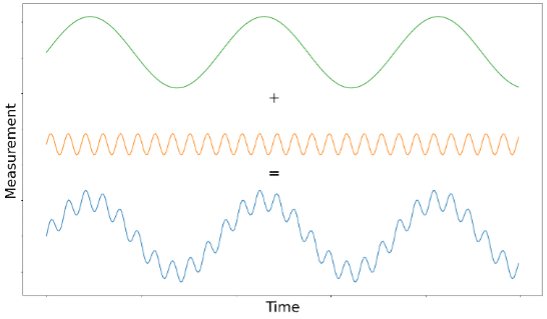
Let’s first broaden our understanding of time series. Time series data is typically collected at a specific rate called sampling rate or frequency which is expressed in Hertz (Hz), the number of values per second. The higher the sampling frequency, the more measurements which in turn means more data. When we plot this data on a graph with the value of the measurement on the y-axis and the time of measurement on the x-axis, we get something like the figure below. Since time is on the x-axis time series lingo considers this display of the data to be in the time domain.

Time vs Frequency-domain
More than 200 years ago the mathematician Joseph Fourier came to the realization that any time-series signal is a combination of simple sine waves with different frequencies and amplitudes. He then came up with a transformation function to decompose a raw signal into the frequencies and amplitudes of the different sine waves it’s made up of. This operation became known as the Fourier Transform.

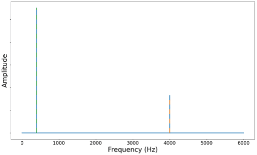
Retaking the original time-based signal and applying a Fourier Transformation to this signal, we can see that our time series originates from 2 sine waves. A first (green) sine wave with a low frequency and high amplitude while the second (orange) has a much higher frequency and lower amplitude. We can plot these frequencies on the x-axis and their associated amplitude on the y-axis to get the figure below. This shows the measurement in the frequency domain as the x-axis represents frequencies instead of time.

Amplitude over frequency plots like the one above display are said to display the signal in the frequency domain while the original signal was in the time domain.
If we want to move back from the frequency domain into the time domain there is a different transformation to do the trick, it’s aptly named the Inverse Fourier Transform.
Introducing synthetic anomalies
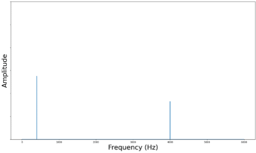
As mentioned in the introduction, some of our industrial clients want to perform anomaly detection on new machines that will be operational for years to come but haven’t behaved anomalously just yet. Rather than wait for things to break, we want to be proactive and create anomalous data ourselves. The Fourier Transform will play a vital role in this. Now that we can go from the time domain to the frequency domain and back, we have an opportunity to tamper with specific frequencies. If we retake figure 3 from above, we see that the signal has 2 important frequencies. The first frequency (green) is around 400Hz, and the second (orange) is around 4000Hz. If we use the amplitude at 400Hz with a factor of 50% we have manually introduced an anomaly at this frequency. Our altered time series in the frequency domain is shown in figure 4. The factor 50% is chosen arbitrarily and can be substituted by any value which increases or decreases the amplitude.

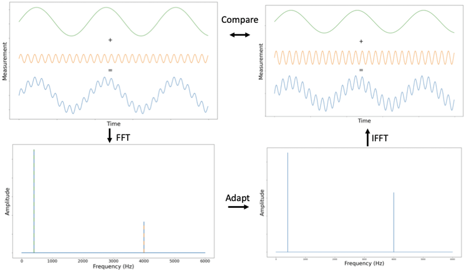
Once we’ve got our new time series in the frequency-domain we can reconstruct the time-based signal by applying the Inverse Fourier Transformation. This is what we’ve done to construct figure 5. We can easily compare the original and the synthetic time series and see that the amplitude of the long waves (400Hz) has decreased while the short waves (4000Hz) have stayed the same, which is exactly what we tried to achieve.

If we recap all steps to introduce synthetic anomalies, we start from a time series in time-domain. We apply a Fourier Transformation on the time series to decompose the signal in its sine wave components where each sine wave has a specific amplitude and frequency. We can adapt the amplitudes of specific sine waves to create a synthetic signal in the frequency domain. The last step is to do an Inverse Fourier Transformation to reconstruct the adjusted time series in the time-domain. This gives us a time series with manually introduced anomalies.

Anomaly detection benchmarking using synthetic anomalies for time series
Now that we have anomalous data, we can test our approach of normality modelling. We train a model on normal data with the task of predicting the signal in the near future.

Once our model is trained, we can use it to predict the future just like a time series forecasting model. In the figure below we show the forecast predictions made by the model compared to the normal measured data. The red line at the bottom shows the Root Mean Squared Error (RMSE) between the prediction and actual data. You can see in increase when the prediction and actual data don’t match very well.

To verify whether our model can detect anomalies, we can introduce synthetic anomalies using the method described in the previous paragraph. Instead of altering the entire signal we decided to only alter a small portion of the signal as this could show the difference between normal and abnormal data. The signal (blue line) between the 2 black vertical lines in figure 8 is altered compared to the signal in figure 7. In other words, this section of the signal contains anomalies and is used as input for the time series forecasting model. This model gives the orange line as predicted values which is closer to the non-altered signal than to the altered signal.

We can clearly see that the RMSE (red line) is higher when there are anomalies. Using a threshold value, visible as the green horizontal line in figure 8, we can search for periods where the error surpasses this threshold for multiple consecutive periods in time. When this is the case, we can binary classify this region as anomalous, validating our approach.
Conclusion
Anomaly detection is a well-studied topic in machine learning which can be applied to many industrial applications. We’ve seen a recurring issue in industry, an abundance of normal data but lack of anomalous data.
To overcome this, Faktion has come up with an approach to create synthetic anomalous data. We managed to validate that our normality modelling approach is capable of separating these synthetic anomalies from the healthy day, allowing us to help our customers detect anomalies that are yet to come. If your company has similar challenges, do not hesitate to contact us, as there is the possibility that we can help you!

